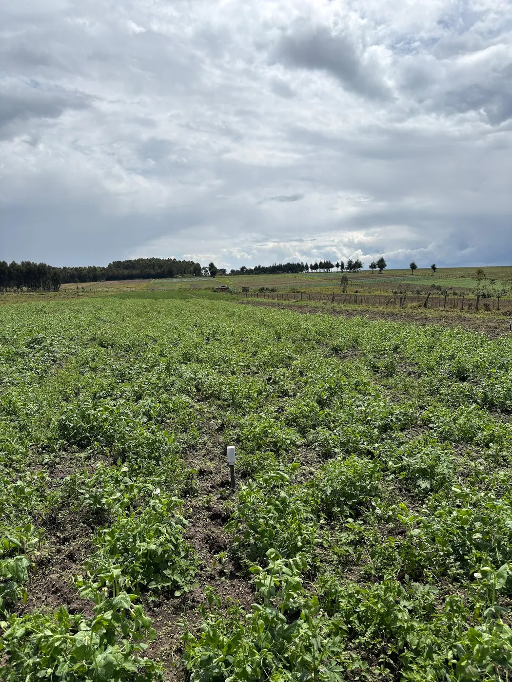
The free app colours the plot green, and the plot is not green
The pitch for satellite crop monitoring comes in one sentence, and it sounds free: draw your field in an app and a satellite will watch it for you. On a large, square field growing a single crop, with nothing around it, that sentence is close to true. Put it on a five-acre plot with a murram track down one side, trees on the boundary and a neighbour growing something else over the fence, and it fails in a particular way. That failure is worth understanding before you decide what, if anything, to pay for.
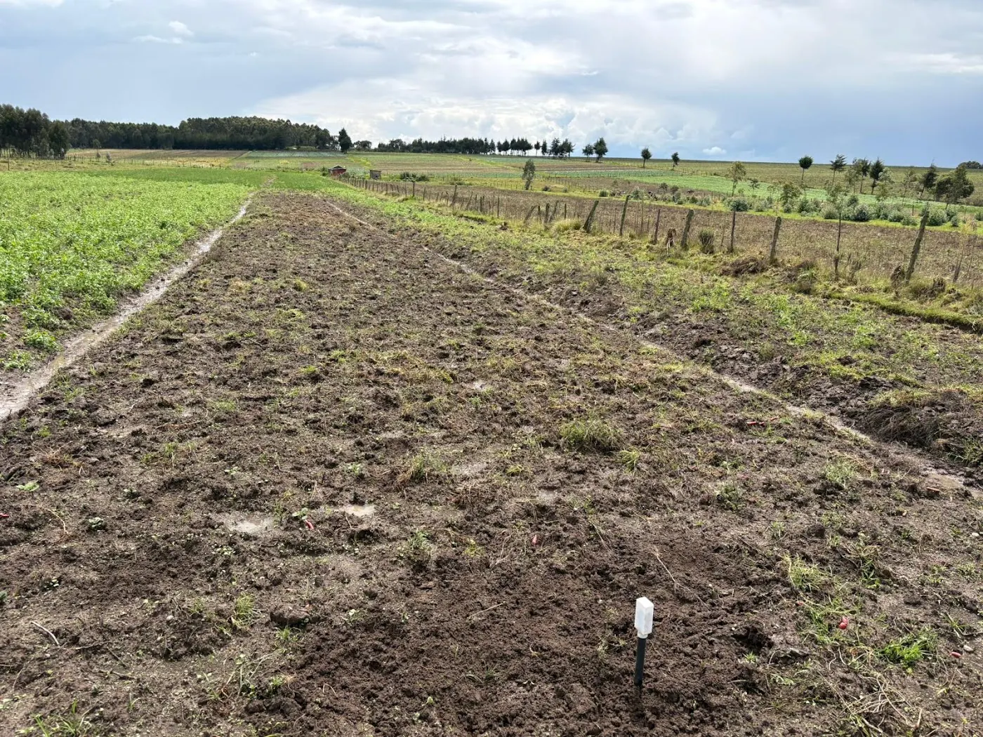
Picture what comes back on the phone. A uniform green rectangle, a number in the corner. The grower walks the field that same afternoon and finds a wilting band along the lower edge, and a bare strip where the planter skipped. Nobody lied. An index averages light bounced off a few dozen squares of ground, and each square holds some crop, some soil, and along the boundary some track and some of the neighbour's field.
The computer science department at Cambridge put the core problem plainly in its note on bringing satellite crop monitoring to the world's most vulnerable farms: small farms are nearly invisible from space, because their fields are tiny and ill-defined, and the tools were designed for the large uniform fields of industrial agriculture rather than sub-hectare plots. Everything below is the detail behind that sentence.
A ratio of two colours of light
Start with what the satellite actually sees, because the index rests on one physical fact. NASA's Earth Observatory explainer on measuring vegetation lays it out: chlorophyll in a leaf strongly absorbs visible light from 0.4 to 0.7 micrometres, while leaf cell structure strongly reflects near-infrared light from 0.7 to 1.1 micrometres. A living canopy therefore looks dark in the visible band and bright in the near-infrared. Bare soil, a track or a dead crop shows no such contrast.
NDVI turns that contrast into a single figure: near-infrared minus visible, divided by near-infrared plus visible. Values run from minus one to plus one. NASA gives the landmarks. Rock, sand or snow sits at 0.1 and below; shrub and grassland at 0.2 to 0.3; temperate and tropical rainforest at 0.6 to 0.8. No crop is measured. No leaf is counted.
Extension uses a tighter band for crops. Alabama Extension's guide to vegetation indices in precision agriculture puts healthy crops typically between 0.6 and 0.9, with stress from disease, drought or nutrient deficiency able to push values below 0.4. A reading of 0.7 over a Kenyan plot says the canopy reflects like dense green vegetation. It does not say whether that vegetation is your maize, the weeds between the rows, or the napier along the fence. Alabama is also candid about the ceiling: in dense crops, early stress might not be detected at all, because a canopy that is already thick keeps the ratio high while the problem begins underneath it.
Reflectance first, index second, the crop a long way third
What the sensor records and what the app sells are further apart than the marketing admits. A paper on open-source software for satellite-based crop health monitoring in the Journal of Biosystems Engineering states it directly: an optical satellite sensor captures crop surface reflectance but does not provide direct measurements of biophysical properties such as NDVI. Someone computes the index afterwards, on the ground, in software a phone user never sees.
That paper describes two of the hidden steps. Radiometric calibration against a reference reflectance target was used to detect and correct abnormalities in the images, because the brightness a satellite records depends on the atmosphere and sun angle as much as on the crop. And the pipeline had to be refined to filter unusable data, including multiples of clipped images and duplicates of tile images, before any analysis ran. Clipped and duplicated tiles are what the raw feed looks like.
Next is the jump from an index to the crop itself. That is the step growers care about, and the step the science is least sure of. A review of challenges in remote sensing-based crop monitoring finds that satellite-derived metrics do not fully capture what drives crop production and do not quantitatively interpret crop growth status. Two things limit real decisions, it says: access to ground data, and the harm done by analyses that lean on expert assumption instead of measurement. Sunlight bounces off a canopy, a sensor records two bands, a pipeline computes a ratio, someone decides what it means. Every link adds doubt. The app shows you only the last one, coloured green.
Five acres, counted in pixels
Now for the arithmetic that decides whether the image can see inside your plot at all. The Journal of Biosystems Engineering paper lays out the spread across agricultural satellites: pixel sizes from 3 to 30 metres, and revisit intervals from daily to 16 days. Convert the plot first. An acre is about 0.4 hectares, so five acres is about 2 hectares. A hectare is 10,000 square metres, which puts the plot at roughly 20,000 square metres.
A 30 metre pixel covers 30 times 30, or 900 square metres. Divide 20,000 by 900, and the coarse end of the free range gives you about 22 pixels for the whole plot. A 3 metre pixel covers 9 square metres, so the fine end gives about 2,200. That 3 metre figure belongs to Planet Scope. The same paper describes it as daily imagery at 3 metre resolution across various spectrums, and it is a commercial product. NASA's AVHRR vegetation pixel is 1 square kilometre. NASA notes that is 100 hectares in one data point. Two hectares into 100 is one fiftieth. At that scale your plot is not a field in the image. It is a rounding error inside one square that also holds the road, the river line, the school compound and dozens of your neighbours.
Twenty-two squares is all a 30 metre product knows about your plot. Picture a sheet of paper torn into twenty-two pieces. That is the resolution at which it will tell you where the wilting band is. Commercial satellites the same paper lists, at 0.3 to 0.5 metres, would see far more. But nothing in the sources puts those prices in front of a Kenyan grower on a phone, so treat them as the upper shelf you are not buying. South Dakota State University's comparison of aerial imagery for crop assessment confirms the free tier: Sentinel-1, Sentinel-2 and Landsat 8 and 9 come at no charge from USGS and NASA. Some Planet datasets can be reached free through specific programmes or portals such as USGS Earth Explorer. Free sits at the coarse end of the ruler. That is the whole trade, and it is the trade every subscription later in this piece is quietly built on. Hold the 22 squares in mind. Every section from here is about what those squares can and cannot carry.
The edge is where the number goes wrong
On a big field, the boundary pixels form a thin frame around a large interior, and the average barely notices them. On a small field, the frame is most of the picture. Cambridge says it exactly: in the smallest fields almost the whole field is edge. A single satellite pixel can fall across two crops, a track or a hedge, blurring the signal. Lay the 22-pixel plot out as a rough rectangle. Squares on the outside ring touch something that is not your crop, while the squares in the middle are few. Your field average is being pulled by whatever grows on the far side of the fence.
That matters more here than in the places where the tools were built. A Kenyan plot often has trees on the boundary, a footpath worn through it, a strip of a second crop and a fence line of napier or sisal. Each one lands in a pixel and adds its reflectance to yours. Intercropping does the same from the inside. A pixel holding maize and beans returns a ratio that belongs to neither. No source quantifies how much a Kenyan plot's number is shifted by this, and this piece will not invent a figure. What the sources do say is that the effect is strongest exactly where plots are small and irregular. That describes most of the country's farmland.
Cambridge's answer is a model called Tessera, tested on small fields in Austria. It identified most crop types more accurately than methods currently in use, while using 8 per cent of the computing power and none of the hand-tuning. Carry the limits with the result. Austrian small fields are not Kenyan small fields. Identifying what crop is growing is a different task from telling you whether it is stressed. One practical handle survives. Alabama notes that on a field-average timeline, a wide standard deviation bar means conditions vary more across the field, and a short bar means even growth. For a plot that is mostly edge, a wide bar may be your fence line talking. Check the bar before you believe the mean.
Cloud, cadence and the composite
How often a free image arrives is the second half of the resolution question. The answer is less often than the revisit interval suggests. The Journal of Biosystems Engineering paper gives daily to 16 days across platforms, with the daily end belonging to the commercial 3 metre product. Free satellites sit toward the longer interval. That is the schedule for a pass, not for a usable image. An optical sensor needs to see the ground, and a highland afternoon sky in a Kenyan rainy season is often exactly what it cannot see through.
Vegetation products get around cloud by stacking passes. NASA describes daily indices being combined into 8-, 16- or 30-day composites to build maps of where plants are thriving and where they are under stress. A composite is cleaner, but it is also older. A 16-day composite tells you about the best cloud-free moment in the past fortnight or so, not about yesterday. For a county drought map that is fine. For a decision about which block to irrigate on Monday, it is already history.
Cloud is the reason the South Dakota comparison carries two alternatives. Airplane imagery can be flown on a customisable path and timed for clear weather, which makes it useful where cloud is frequent; it also carries flight permissions, limited coverage, weather dependency and higher cost than satellites. Drones fly under the cloud entirely, and a later section returns to them. On the free route, expect gaps and expect composites. And do not read a number dated three weeks ago as a report on the field you walked this morning.
The anomaly, not the colour, is the drought signal
If the absolute number cannot see inside the plot, what is a free vegetation index good for? Comparison over time. That is a better use than most apps advertise. NASA defines the NDVI anomaly as the difference between the average NDVI for a month in a given year and the average NDVI for that same month over the last twenty years. Vegetation growth in most climates is limited by water, NASA adds, so relative vegetation density is a good indicator of agricultural drought. A pixel that is browner than its own long-run average for that month says something a single green number never can.
National agencies have made this use formal. FAO's guidelines on using remote sensing products for early warning exist to help countries put freely available imagery and derived agro-climatic indicators to work in warning systems. That is a county and national scale tool. It will tell a ministry that a region is browner than usual for November. It will not tell you which of your blocks is short of water.
A satellite rainfall product shows the same strength and the same limit. CHIRPS is a satellite-and-gauge rainfall record, not one of our gauges, and for the grid cells where NuaSense stations stand it gives a long-term November average of 114 mm across 43 years from 1983 to 2025, with a driest November of 47 mm in 1983 and a wettest of 290 mm in 2019. That is a usable baseline for an anomaly. Set it against what the ground recorded: over 09 October to 08 November 2026, totals at individual NuaSense stations ranged from 0.0 mm to 122.7 mm across 14 stations. Those stations are not co-located, and the spread is not a regional figure. It is a measured illustration of how much variation a single composite pixel averages away. An anomaly tells you the region's season is unusual. A gauge, or a walk, tells you whether yours is.
Water in the index is not water in the plant
NDVI is the index most apps lead with, but it is one of a family, and the water one deserves its own warning. Alabama gives thresholds for NDMI, the moisture index: below 0.1 indicates significant water stress, below 0.2 suggests possible water stress or low canopy cover, and above 0.4 shows good canopy with no water stress. Then it takes the thresholds back in the next breath. NDMI does not measure how much water is inside the plants. Changes in the index only show which parts of the field might be getting too dry, and it captures average conditions over time rather than rapid short-term moisture changes. Notice the overlap too: a low value can mean stress or simply thin canopy. The image cannot tell which.
That is the whole case for keeping ground measurement in the loop. Alabama's guidance is explicit that growers should always scout the field to confirm what remotely sensed data shows, by examining soil, analysing plant leaves or checking for pests. An index is a pointer to where to walk. For the pest half of that list, the crop protection section of this site covers what to look for once you are standing in the row.
Here is where a buried probe fits. A NuaSense soil sensor reads moisture roughly every ten minutes at a shallow and a deeper depth, as percent of sensor scale rather than calibrated volumetric water, and sends it over LoRaWAN to the weather station. That is the opposite of the satellite: one spot read constantly, instead of the whole plot read occasionally. Where the walk keeps finding trouble in the same corner, a probe there answers the question the image raised. Our dashboard shows a farm's own readings next to public satellite crop condition and rainfall, free to read at agriculture-data.com; the cost is the hardware, never the data. The NuaSense post on IoT applications in Kenyan agriculture covers which low-cost sensor types smallholders are actually using and how the phone-based platforms around them work.
The price ladder run against five acres
Three prices appear in the Journal of Biosystems Engineering paper, and the gap between them is the lesson. EOS charges 1.5 US dollars per acre for a monitoring platform built on Landsat, Sentinel and SuperView imagery. Farmers Edge sits at 2 to 4.5 US dollars per acre, depending on the service level. DynaCrop, which delivers vegetation and leaf area indices through a web portal, runs to 999 euros per month. The paper does not say what billing period the per-acre figures use, so treat them as published.
Now multiply by five. EOS works out at 7.5 US dollars for the plot. Farmers Edge lands at 10 US dollars on the low tier and 22.5 on the high one. DynaCrop's ceiling does not come down at all: 999 euros covers five acres or five thousand, which tells you who it was built for. These are dollar and euro figures from the paper, not shilling prices, and the exchange rate on the day is yours to look up.
Weigh that honestly. A per-acre tier is not expensive. It does not buy you resolution either, because the source imagery it names is the same Landsat and Sentinel that USGS and NASA give away. What you get over five acres is still the 22 squares already counted above, plus drawing tools, a time series and someone else's calibration pipeline. The same paper reports that at the time of writing no open-source analytic software for agricultural satellite imagery was available, which kept the data out of reach of many producers. That is the real thing a subscription sells: software between the raw tile and the number. For a five-acre plot the plain call is this. Start on the free route, look at the anomaly and the spread bar rather than the colour, and walk the field. Pay a per-acre fee only if the portal's time series changes a decision you actually make. Never pay for a 999 euro portal. If the subscription competes with inputs for the same money, a small index over 22 pixels is not the line to protect.
Drones, aircraft and the national programme launched in Nairobi
When the plot is too small for the satellite, the usual next suggestion is a drone, and South Dakota supports part of it. Drones capture very high spatial resolution at centimetre-level precision, and for small to medium-sized farms they are usually cost-effective. Multi-rotor models fly for 20 to 40 minutes. They also face regulatory restrictions on flights in some areas and require expertise in flight planning, data acquisition and processing. In Kenya that regulation sits with the Kenya Civil Aviation Authority, and the permissions are the operator's problem, not a detail to skip. Cost on the same class of equipment is worked through in this site's piece on spray drones against a knapsack, and the hire-rather-than-buy logic there applies to a camera flight over five acres. Cost-effective is not cheap, and the expertise line is where many a hired flight produces a pretty picture nobody can interpret.
The other development is national. Kenya Space Agency reports the launch of the Crop Measurement and Evaluation initiative, CroME, at KALRO headquarters in Nairobi on 10 to 11 February 2026, in partnership with the Ministry of Agriculture and Livestock Development, Microsoft AI for Good Lab and NASA Harvest. The intended outputs are crop maps, crop growth monitoring, field boundaries, yield predictions, crop damage detection and disaster early warning. Read that list against everything above. Field boundaries and crop maps are the exact problem Cambridge named, and a national effort to draw Kenyan boundaries properly is the most useful item for a small plot. Yield prediction is the item the review warned satellite metrics cannot do quantitatively on their own. The source describes a launch and intentions, not delivered products, and nothing in it says when a five-acre farmer sees an output. Your plot will still be 22 squares with a hedge in the outer ring, and the afternoon walk along the lower edge will still be the instrument that catches what the squares averaged away.